OMPS-NPP NASA – WP

This page documents the application of the Complete Data Fusion (CDF) algorithm to the OMPS / SUOMI-NPP ozone profile product. OMPS (Ozone Mapping and Profiler Suite) Nadir Profiler retrieves ozone vertical profiles from UV backscatter measurements on a coarse 20-layer grid. A distinctive feature of this dataset is that the file explicitly stores the Jacobian matrix K (sensitivity of UV radiances to ozone per layer), enabling two independent reconstructions of the averaging kernel and error covariance: one read directly from the file and one derived from K and an external measurement error model. Both variants are tested.

1. Overview

Provider	NASA — National Aeronautics and Space Administration (Goddard Space Flight Center / GES DISC)
Instrument	OMPS-NP (Ozone Mapping and Profiler Suite — Nadir Profiler) — UV backscatter spectrometer, ~250–310 nm, ground pixel ≈ 250 km × 250 km
Platform	SUOMI-NPP (Suomi National Polar-orbiting Partnership) — sun-synchronous polar orbit, ≈ 824 km altitude, 13:30 equator crossing (ascending)
Product	OMPS/NPP NP Total Column and Profile Ozone L2 (`OMPS_NPP_NPBUVO3_L2`)
Retrieval algorithm	BUV optimal estimation — profile retrieval in 20 pressure layers from UV backscatter in 10 spectral channels
Tested constituent	O₃ (ozone profile)
File format	HDF5 (non-CF)
CDF reader	`OMPSHdf5NadirReader` (`cdftools.readers.omps_hdf5_nadir_reader`)
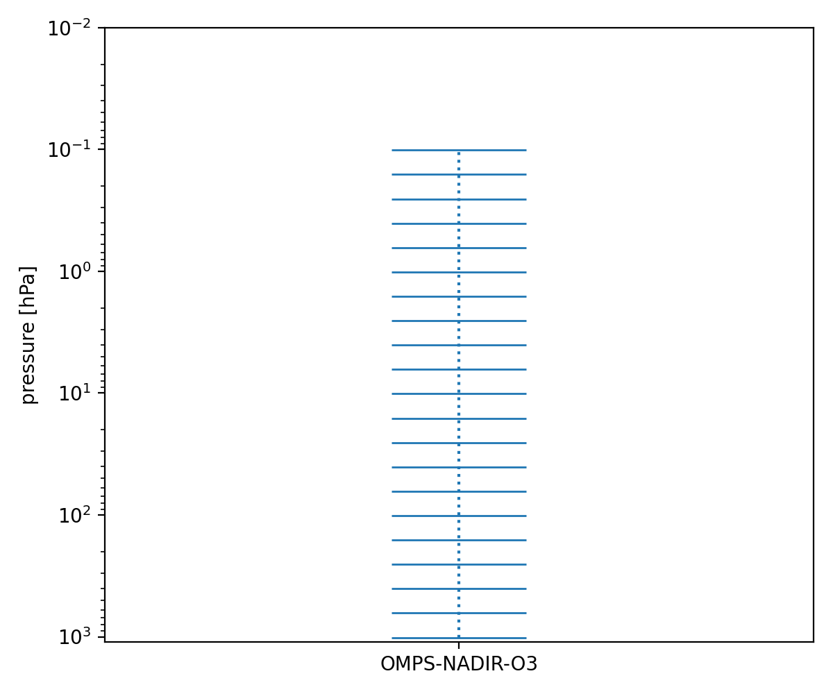
Vertical grid	20 pressure layers (DimPressureLevel20) — layer centers · 21 pressure levels (DimPressureLevel) — layer bottoms
Spectral channels	10 UV backscatter channels used in retrieval (Jacobian K: 20 × 10)
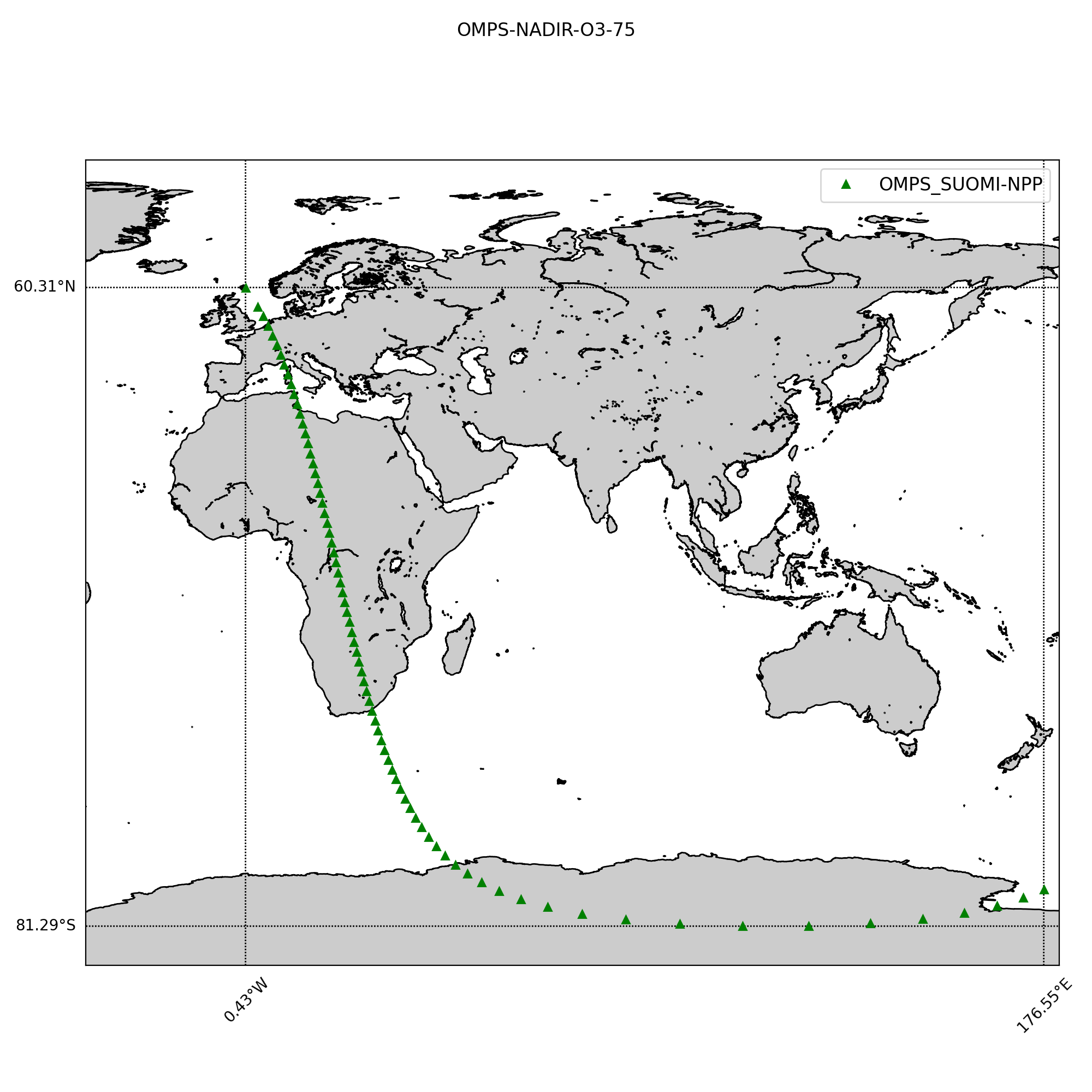
Test granule	SUOMI-NPP, orbit 42295, 2019-12-26 11:35 UTC
CDF status	Tested — CDF(2022) passes for Variant A (AK from file); CDF(2015) fails for both variants (see §7)

2. FAIR References

OMPS/NPP NP L2 data are publicly available at no cost from the NASA GES DISC archive (NASA Earthdata account required). Metadata verified on 2026-04-11 from the test file attributes and filename convention.

Product title	OMPS/NPP NP Total Column and Profile Ozone L2 2-d Swath 1 Orbit ~100 min
Short name / version	`OMPS_NPP_NPBUVO3_L2` version 2.8
Data access	NASA GES DISC — OMPS_NPP_NPBUVO3_L2_V2
Institution	NASA Goddard Space Flight Center (GSFC), Greenbelt, MD, USA
Algorithm reference	McPeters, R. D. et al. (2019): Total column ozone retrievals from the SNPP OMPS satellite instrument. J. Geophys. Res. Atmos., 124, 1528–1544. doi:10.1029/2018JD029576
License	NASA open data policy — free for scientific use; registration at NASA Earthdata required for access
File naming convention	`OMPS-NPP_NPBUVO3-L2_v{ver}_{YYYYmMMDDtHHMMSS}_o{orbit}_{processing_date}.h5`
Contact	NASA GES DISC Help Desk: gsfc-help-disc@lists.nasa.gov

3. Dataset Description

The OMPS Nadir Profiler (NP) retrieves ozone vertical profiles by measuring UV backscatter radiation from the Earth’s atmosphere and surface. Unlike the Total Column instrument, the NP uses longer UV wavelengths (300–310 nm) that penetrate deeper into the troposphere, yielding a coarse vertical profile on a fixed 20-layer pressure grid.

The retrieval algorithm is a BUV (Backscattered UV) optimal estimation scheme. The measurement vector consists of 10 UV radiance ratios at specific wavelengths; the state vector is the ozone partial column in each of the 20 pressure layers. The Jacobian matrix K (∂radiance/∂ozone, dimensions 20 × 10) is stored explicitly in the HDF5 file, making this one of the few satellite products that ships K alongside the retrieved profile, AK and error information.

Key characteristics of the error representation in this product:

Averaging kernel (AK): stored directly as a 20×20 matrix in ScienceData/AveragingKernel.
Total covariance from AK: not stored; reconstructed as S_tot,AK = (I − AK) · S_a.
Total covariance from K: reconstructed as S_tot,K = (K · S_M⁻¹ · K^T + S_a⁻¹)⁻¹, where S_M = (1%)² · I₁₀ is the assumed measurement error covariance for 10 UV channels.
A priori covariance S_a: not stored in the file; constructed by the reader as a relative covariance with standard deviation equal to the a priori profile value and an exponential correlation function with length scale of 3 layers.

Both the file-stored AK and the K-derived AK are tested independently to assess whether the two representations are mutually consistent with the CDF framework.

4. State Vector and Vertical Grid

The state vector is the ozone partial column (in Dobson Units, DU) in each of the 20 pressure layers. The vertical grid is defined by 21 pressure levels (DimPressureLevel), which are the bottoms of the solution pressure levels; the layer centres are stored separately in DimPressureLevel20. The topmost two levels are merged in the reader (the last element of the retrieved 21-value array is added to the second-to-last), yielding a 20-element state vector:

x21 = ScienceData/ProfileO3Retrieved   # shape (N, 21)
x   = x21[:, :-1]                       # first 20 elements
x[:, -1] += x21[:, -1]                  # merge top layer into layer 19
# same for xa = AncillaryData/ProfileO3APrioriLayer

OMPS/NPP ozone — vertical pressure grid — Fig. 1 — OMPS/NPP ozone 20-layer pressure grid and retrieved O₃ profile for a representative product in the test granule.

5. Test File

Filename	`OMPS-NPP_NPBUVO3-L2_v2.8_2019m1226t113528_o42295_2021m0530t202504.h5`
Sensing time	2019-12-26 at 11:35:28 UTC
Platform / orbit	SUOMI-NPP, orbit 42295
Processing date	2021-05-30
Pixels in file	80 total along-track scans (DimAlongTrack = 80)
Quality filter	`ProfileO3ErrorFlag = 0` (ascending orbit, full quality) or `= 10` (descending orbit, also accepted)
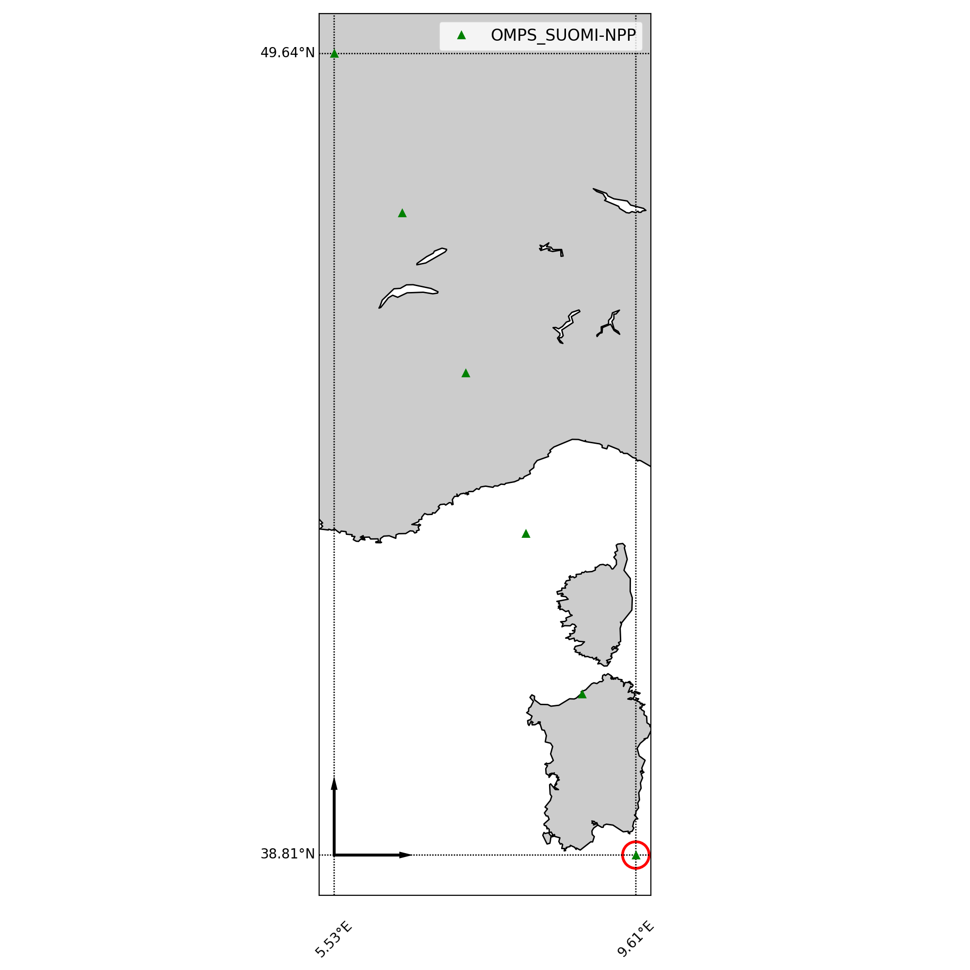
Test area (zoom)	Central Italy and surroundings — box centred at 43.75°N, 11.25°E, ±7° in both directions
CDF test script	`scripts/05_PNRR_filetest/07_OMPS_NADIR.py`

OMPS/NPP ozone — granule coverage map — Fig. 2 — Geographic distribution of good-quality products in the test granule (orbit 42295, 2019-12-26). Dots are sized by retrieved O₃ column.

OMPS/NPP ozone — zoom map central Italy — Fig. 3 — Zoom on the central Italy area (36.75–50.75°N, 4.25–18.25°E) showing the large OMPS-NP ground pixels (≈ 250 km × 250 km). The circle marks the nearest-neighbour distance for the selected product; the arrow indicates the along-track scan direction.

6. Completeness Test Results

The completeness test checks that for each product passing the quality filter the state vector (20 values), a priori profile (20 values), averaging kernel (20×20), and all derived covariance matrices are fully populated and finite.

Test	Result
Products passing quality filter (`ProfileO3ErrorFlag ∈ {0, 10}`)	Subset of the 80-pixel granule (ascending and descending orbit footprints)
State vector completeness (`o3`, 20 levels)	PASS
A priori completeness (`o3_apriori`, 20 levels)	PASS
AK from file (20×20) — positive definite	PASS
AK from K (20×20) — positive definite	PASS
S_a (20×20) — positive definite	PASS
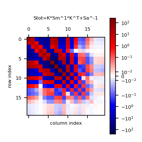
S_tot,AK = (I − AK) · S_a — positive definite	PASS — see Fig. 4
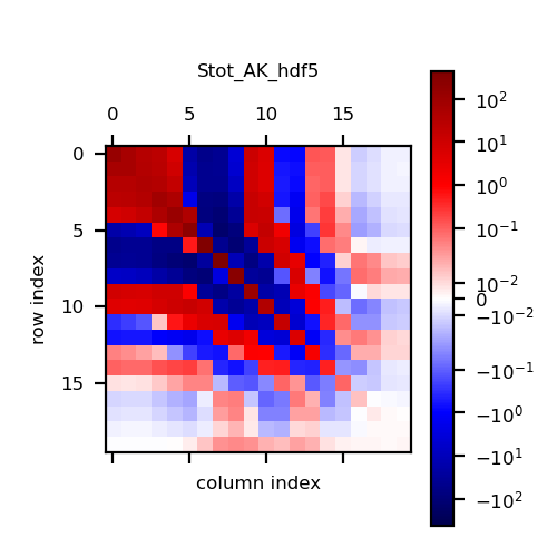
S_tot,K = (K · S_M⁻¹ · K^T + S_a⁻¹)⁻¹ — positive definite	PASS — see Fig. 5

OMPS/NPP O3 — AK from file (rows) — Fig. 4a — AK rows from `ScienceData/AveragingKernel`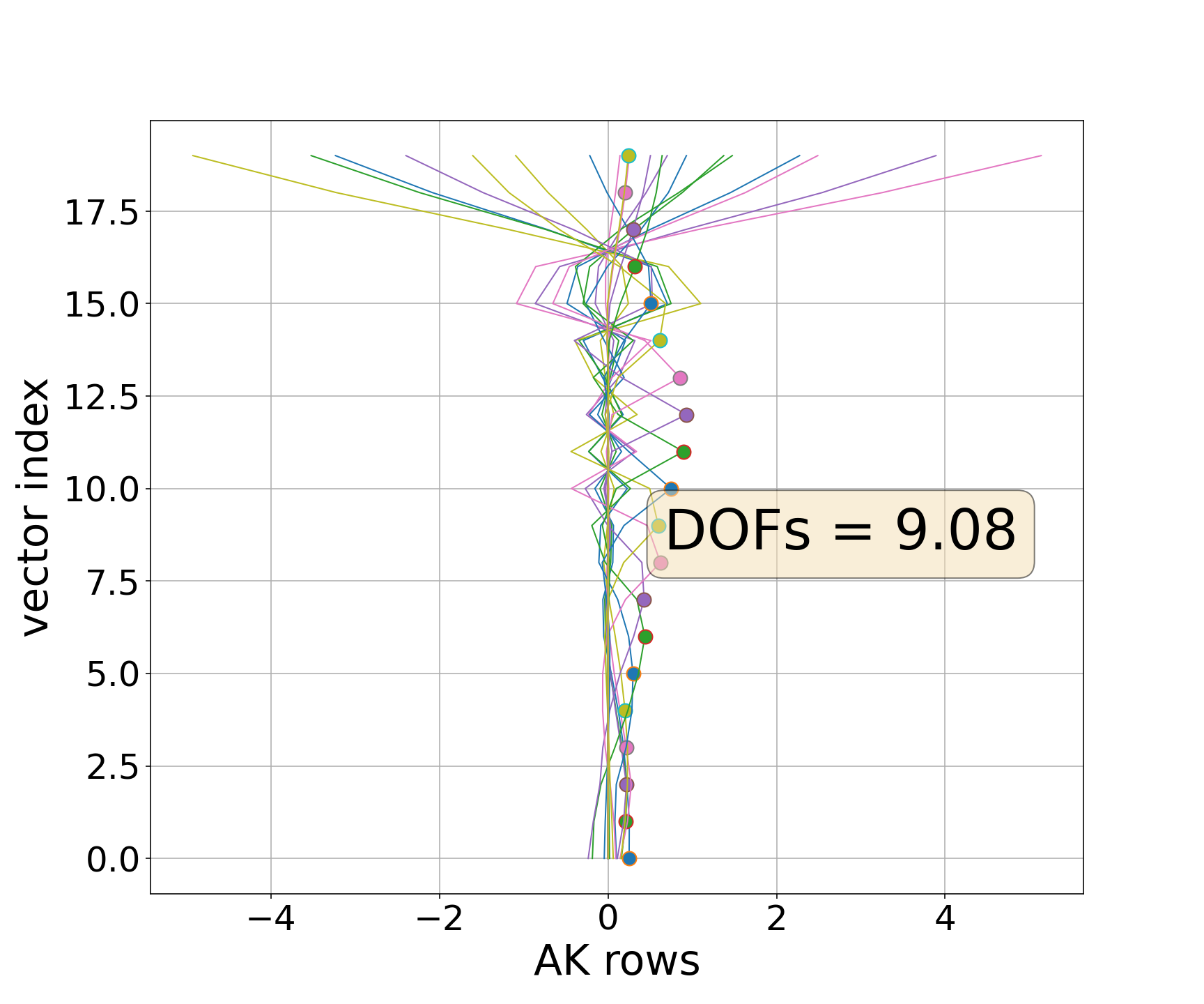

OMPS/NPP O3 — AK from K — Fig. 4b — AK rows reconstructed from Jacobian K

OMPS/NPP O3 — Stot from AK — Fig. 5a — S_tot,AK = (I − AK) · S_a

OMPS/NPP O3 — Stot from K — Fig. 5b — S_tot,K = (K · S_M⁻¹ · K^T + S_a⁻¹)⁻¹

7. Auto-consistency Test Results

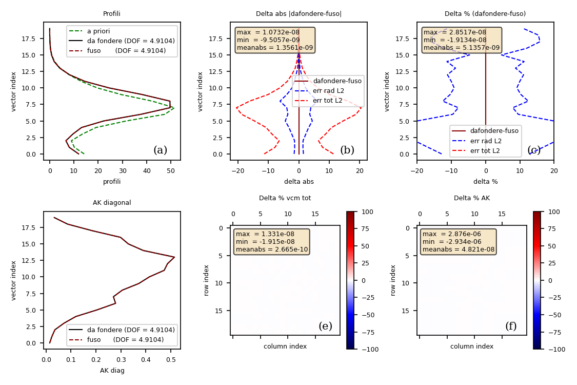
Two independent auto-consistency tests are performed, corresponding to the two representations of the averaging kernel and error covariance. In both cases a single representative product is selected (the first good-quality pixel in the zoomed area around central Italy).

7.1 Variant A — AK from file (`ScienceData/AveragingKernel`)

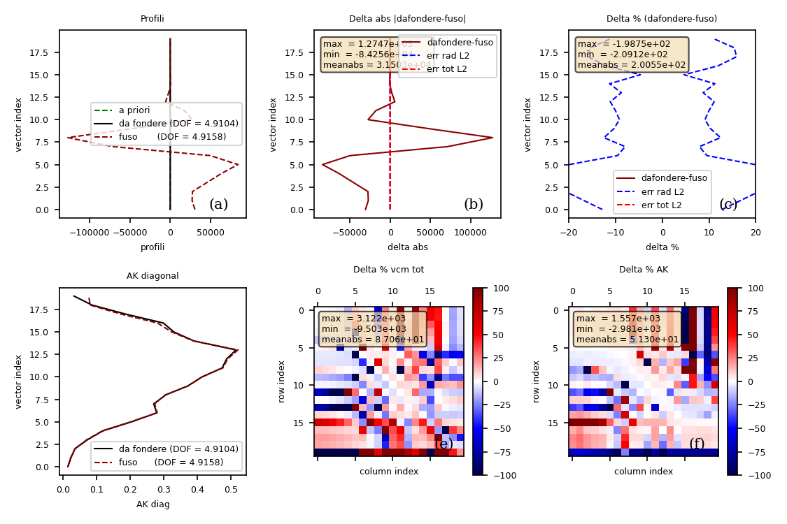
Uses the AK stored directly in the file. The total covariance is reconstructed as S_tot,AK = (I − AK) · S_a, and the noise covariance as S_ε,AK = AK · S_tot,AK. CDF(2022) uses rcond = 0; CDF(2015) uses rcond = 1×10⁻¹¹. CDF(2022) passes; CDF(2015) fails due to poor conditioning of S_ni (non-symmetric S_i from AK-based reconstruction).

#	OMPS-NPP-O3 Auto-consistency test results — Variant A	$\max(\|\Delta x\|)\%$	$(\|\Delta\mathrm{DOFs}\|)\%$
1	CDF(2022) total error VCM inversion	<0.000001	0.000009
2	CDF(2015) noise error VCM inversion	209.120240	0.111199

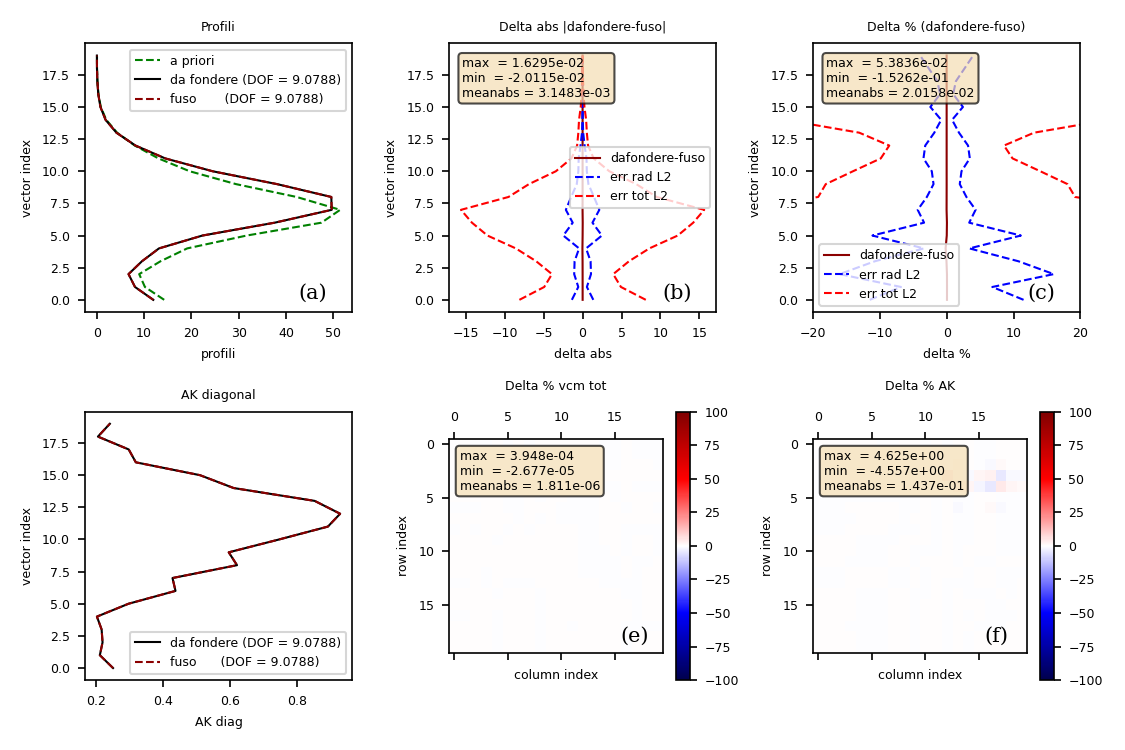
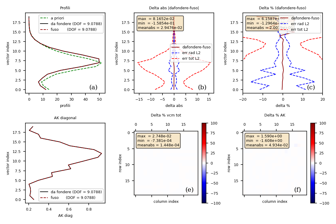
OMPS O3 auto-consistency AK CDF(2022) — Fig. 6a — CDF(2022), Variant A (AK from file)

OMPS O3 auto-consistency AK CDF(2015) — Fig. 6b — CDF(2015), Variant A (AK from file)

7.2 Variant B — AK from Jacobian K

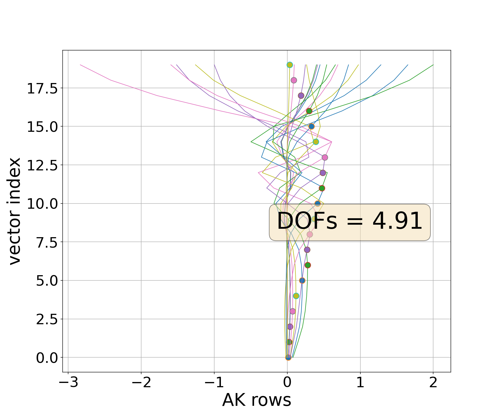
Uses the AK reconstructed from the Jacobian: AK_K = I − S_tot,K · S_a⁻¹, where S_tot,K = (K · S_M⁻¹ · K^T + S_a⁻¹)⁻¹ and S_M = (1%)² · I₁₀. CDF(2022) uses rcond = 0; CDF(2015) uses rcond = 1×10⁻¹². In this variant the VCMs are symmetric but the AK matrix differs significantly from the one stored in the file; the resulting DOFs value (9.08) is inconsistent with the expected value of ~5 found in the literature. Both CDF(2022) and CDF(2015) fail.

#	OMPS-NPP-O3 Auto-consistency test results — Variant B	$\max(\|\Delta x\|)\%$	$(\|\Delta\mathrm{DOFs}\|)\%$
1	CDF(2022) total error VCM inversion	0.152621	<0.000001
2	CDF(2015) noise error VCM inversion	12.963737	0.000004

OMPS O3 auto-consistency K CDF(2022) — Fig. 7a — CDF(2022), Variant B (AK from K)

OMPS O3 auto-consistency K CDF(2015) — Fig. 7b — CDF(2015), Variant B (AK from K)

8. CDF Variables Mapping

CDF quantity	Reader attribute	HDF5 path	Units / notes
State vector x	`p.o3`	`ScienceData/ProfileO3Retrieved`	DU per layer (21 values → collapsed to 20 by merging top layer)
A priori x_a	`p.o3_apriori`	`AncillaryData/ProfileO3APrioriLayer`	DU per layer (same collapsing as state vector)
Pressure — layer centres	`p.pressure_layer_center`	`DimPressureLevel20`	hPa; 20 values; common to all pixels in file
Pressure — layer bottoms	`p.pressure`	`DimPressureLevel`	hPa; 21 values; layer boundary pressures
Averaging kernel (from file)	`p.ak`	`ScienceData/AveragingKernel`	20×20; axes transposed by reader (file stores as [along_track, dim20, dim20] with rows/cols swapped)
Jacobian matrix K	`p.K`	`ScienceData/KMatrix`	20 × 10 (profile levels × UV channels); ∂radiance/∂ozone
A priori covariance S_a	`p.vcm_a`	— (not in file)	Constructed by reader: S_a[i,j] = √0.5 · x_a[i] · x_a[j] · exp(−\|i−j\|/3); relative covariance, σ ≈ 70%, correlation length 3 layers
Total covariance (AK-based)	`p.vcm_tot_ak`	— (computed)	S_tot,AK = (I − AK) · S_a
Total covariance (K-based)	`p.vcm_tot_K`	— (computed)	S_tot,K = (K · S_M⁻¹ · K^T + S_a⁻¹)⁻¹; S_M = (1%)² · I₁₀
AK reconstructed from K	`p.ak_K`	— (computed)	AK_K = I − S_tot,K · S_a⁻¹
Noise covariance (AK-based)	`p.vcm_ak`	— (computed)	S_ε,AK = AK · S_tot,AK
Noise covariance (K-based)	`p.vcm_K`	— (computed)	S_ε,K = AK_K · S_tot,K
Quality flag	—	`ScienceData/ProfileO3ErrorFlag`	Accepted: 0 (ascending, good) or 10 (descending, acceptable)
Orbit number	—	`attrs['OrbitNumber']`	HDF5 global attribute

9. Notes and Open Issues

S_a not stored in file. Unlike most other datasets tested, the OMPS NP product does not include the a priori covariance matrix in the distributed file. The reader constructs S_a as a relative covariance from the a priori profile using an exponentially decaying correlation function with length scale of 3 layers and a scaling factor k = √0.5 (approximately 70% relative standard deviation). This construction is consistent with the algorithm description in the NASA Product Generation Specification but is not a verbatim reproduction of the operational S_a.
Two AK representations compared. The file-stored AK (Variant A) and the K-derived AK (Variant B) produce slightly different auto-consistency results due to the approximations in S_M (assumed 1% measurement error). The comparison of Figs. 6 and 7 shows how sensitive the CDF results are to the choice of error representation.
Coarse 20-layer grid. The OMPS NP retrieval uses only 20 pressure layers from the surface to the upper stratosphere, a much coarser vertical sampling than IASI (101 levels) or MIPAS (27 levels). The CDF test in profile space is therefore computationally lightweight (20×20 matrices), but the vertical resolution of the fused product will be limited by this grid.
Jacobian K stored in file. The availability of K (20×10) enables a first-principles reconstruction of the error covariance without relying on the file-stored AK. This is a useful cross-check and makes OMPS NP one of the more self-consistent datasets for CDF purposes.
Measurement error model. The measurement error covariance S_M = (1%)² · I₁₀ is a diagonal approximation assuming uncorrelated 1% radiance errors in each of the 10 UV channels. The NASA algorithm documentation notes that for operational processing this is increased to 2%. The impact of this choice on the CDF results has not been quantified.
OMPS Limb Profiler not tested. OMPS also includes a Limb Profiler (LP) instrument with much finer vertical resolution (≈ 2 km). CDF testing on the LP product is planned but not included in the current version of this page.